
In Apache Spark, efficient data management is essential for maximizing performance in distributed computing. Partitioning, repartitioning, and coalescing actively govern how data organizes and distributes across the cluster. Partitioning involves dividing datasets into smaller chunks, enabling parallel processing and optimizing operations. Repartitioning allows for the redistribution of data across partitions, adjusting the balance for more effective processing and load balancing. Coalescing, however, aims to minimize overhead by reducing the number of partitions without a full shuffle. While partitioning establishes the initial data distribution scheme, meanwhile repartitioning and coalescing are operations that modify these partitions to enhance performance or optimize resources by redistributing or consolidating data across the cluster. A good knowledge of these operations empowers Spark developers to fine-tune data layouts, optimizing resource utilization and enhancing overall job performance.
What is a Partition in Spark?
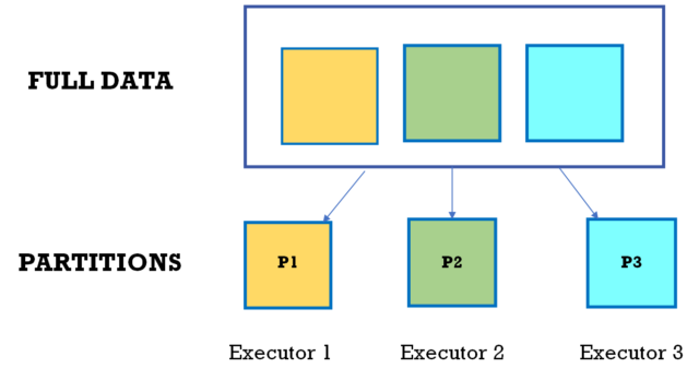
A partition is a fundamental unit that represents a portion of a distributed dataset. It is a logical division of data that allows Spark to parallelize computation across a cluster of machines. Partitions are created when data is loaded into an RDD (Resilient Distributed Dataset) or a DataFrame. Each partition holds a subset of the total dataset, and Spark operations are performed independently on each partition.
In summary, a partition in Spark is a logical unit that facilitates the distribution and parallel processing of data across a cluster. Understanding and managing partitions is crucial for optimizing the performance and resource utilization of Spark applications.
Why Use a Spark Partitioner?
In Apache Spark, partitions play a crucial role in parallelizing and distributing data processing across a cluster of machines. A Spark partitioner determines how the data in a RDD (Resilient Distributed Dataset) or DataFrame is distributed among the available nodes. Using a Spark partitioner is essential for several reasons:
Parallel Processing:
- Partitions enable parallel processing by allowing different portions of the dataset to be processed simultaneously on different nodes of the cluster.
- Each partition operates independently, leading to improved performance and reduced computation time.
Resource Utilization:
- Spark partitions help in efficient resource utilization by distributing the workload across multiple nodes.
- This ensures that the available computational resources, such as CPU and memory, are utilized optimally, leading to better performance.
Load Balancing:
- A well-designed partitioning strategy ensures load balancing, preventing any single node from being overwhelmed with a disproportionately large amount of data.
- Load balancing is crucial for preventing stragglers and maintaining a uniform distribution of work across the cluster.
Shuffling Optimization:
- During operations that require shuffling, like groupByKey or reduceByKey, an effective partitioning strategy minimizes data movement across the cluster, optimizing performance.
- Efficient shuffling reduces the need to transfer large amounts of data over the network, which can be a resource-intensive process.
Join and Aggregation Performance:
- Spark partitions significantly impact the performance of join and aggregation operations.
- A well-designed partitioning strategy can facilitate more efficient join operations, minimizing the need for data movement between nodes.
In summary, the use of Spark partitioners is essential for optimizing data processing in distributed environments. Effective partitioning strategies lead to better parallelism, improved resource utilization, and overall enhanced performance in Apache Spark applications.
Repartition:
Repartition is used to increase or decrease the number of partitions in a DataFrame or RDD by shuffling the data across the cluster. It is particularly useful when you want to explicitly change the count of partitions, perhaps for load balancing or before performing certain operations that benefit from a different partition count.
Example of Repartition:
// Creating a DataFrame
val data = Seq(("John",20),("Alice", 25), ("Bob", 30), ("Charlie", 35))
val df = data.toDF("Name", "Age")
// Initial number of partitions
val initialPartitions = df.rdd.partitions.length
println(s"Initial partitions: $initialPartitions")
// Repartitioning to 2 partitions
val repartitionedDF = df.repartition(2)
// Number of partitions after repartitioning
val partitionsAfterRepartition = repartitionedDF.rdd.partitions.length
println(s"Partitions after repartition: $partitionsAfterRepartition")
-------------------------------------------------------------------------------------
output:
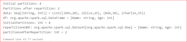
Initial partitions: 4
Partitions after repartition: 2
data: Seq[(String, Int)] = List((John,20), (Alice,25), (Bob,30), (Charlie,35))
df: org.apache.spark.sql.DataFrame = [Name: string, Age: int]
initialPartitions: Int = 4
repartitionedDF: org.apache.spark.sql.Dataset[org.apache.spark.sql.Row] = [Name: string, Age: int]
partitionsAfterRepartition: Int = 2
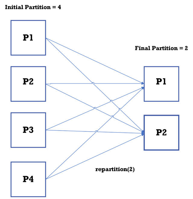
In this example, repartition (2) changes the DataFrame df to have 2 partitions from 4 partitions. Repartition causes a shuffle operation, redistributing the data across the specified number of partitions.
The below data flow diagram shows how repartition works:
Coalesce:
Coalesce is similar to repartition but it can only decrease the number of partitions, and this will not cause any shuffle. It is used for reducing partitions after filtering or similar operations to minimize the number of small partitions and optimize performance.
Example of Coalesce:
// Creating a DataFrame
val data = Seq(("John",20),("Alice", 25), ("Bob", 30), ("Charlie", 35))
val df = data.toDF("Name", "Age")
// Initial number of partitions
val initialPartitions = df.rdd.partitions.length
println(s"Initial partitions: $initialPartitions")
// Coalescing to 2 partitions
val coalescedDF = df.coalesce(2)
// Number of partitions after coalesce
val partitionsAfterCoalesce = coalescedDF.rdd.partitions.length
println(s"Partitions after coalesce: $partitionsAfterCoalesce")
---------------------------------------------------------------------------------
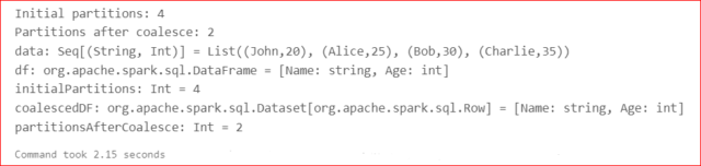
output:
Initial partitions: 4
Partitions after coalesce: 2
data: Seq[(String, Int)] = List((John,20), (Alice,25), (Bob,30), (Charlie,35))
df: org.apache.spark.sql.DataFrame = [Name: string, Age: int]
initialPartitions: Int = 4
coalescedDF: org.apache.spark.sql.Dataset[org.apache.spark.sql.Row] = [Name: string, Age: int]
partitionsAfterCoalesce: Int = 2
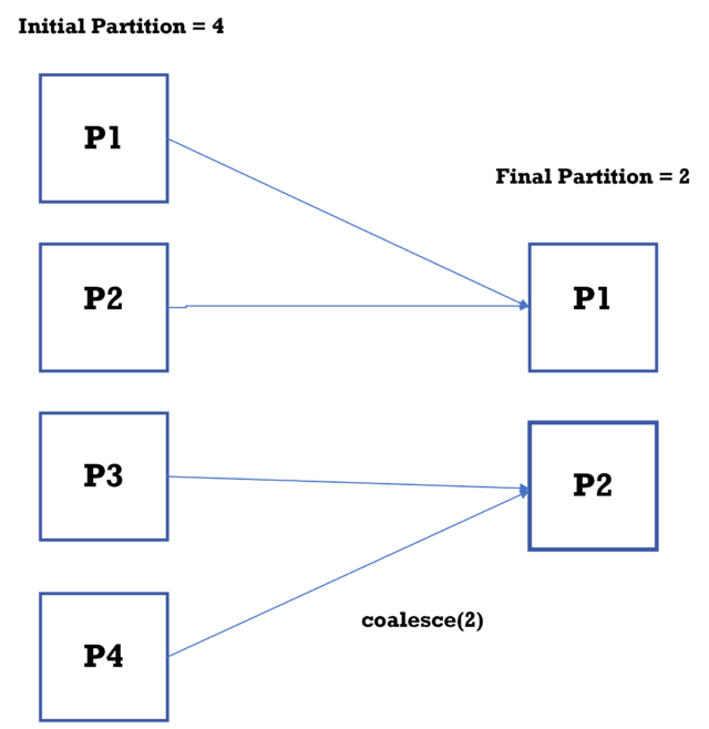
In this example, coalesce (2) reduces the DataFrame df to have 2 partitions from 4 partitions. Unlike repartition, coalesce performs a narrow transformation, minimizing data movement by merging existing partitions whenever and wherever possible.
The below data flow diagram shows how coalesce works:
Difference between repartition and coalesce:
The key differences between repartition and coalesce in Spark lie in their behaviors, performance characteristics, and use cases:
Shuffling:
Repartition: Involves a full shuffle of data across the nodes in the cluster, regardless of whether you are increasing or decreasing the number of partitions. It can be computationally expensive.
Coalesce: Attempts to minimize data movement by merging existing partitions. It doesn’t perform a full shuffle when reducing the number of partitions, making it more efficient.
Number of Partitions:
Repartition: Can be used to both increase and decrease the number of partitions.
Coalesce: Primarily used for decreasing the number of partitions.
Use Cases:
Repartition: Suitable when you want to balance the data distribution across nodes, optimize for parallelism, or explicitly control the number of partitions.
Coalesce: Useful when you want to reduce the number of partitions without incurring the overhead of a full shuffle. It’s often used when the data is already reasonably balanced and doesn’t require significant reshuffling.
Performance:
Repartition: Can be more computationally expensive due to the full shuffle operation, especially when increasing the number of partitions.
Coalesce: Generally, more efficient when decreasing the number of partitions, as it avoids the full shuffle.
Example:
In the below example, the process of repartitioning consumed a longer duration, while coalescing is proving to be more time efficient.
Repartition took: 43.77 seconds
Coalesce took: 2.15 seconds
In conclusion, understanding the concepts of partitioning, repartitioning, and coalescing is crucial for optimizing the performance and resource utilization in Apache Spark applications.
Selecting the appropriate strategy depends on the nature of the data, the computational workload, and the desired level of parallelism. Whether aiming for data balancing, load optimization, or efficient shuffling, understanding these concepts empowers Spark developers to make informed decisions that enhance the overall efficiency of their distributed data processing pipelines.